I first saw a wood elevation map at the World-Class Mountain View Art & Wine Festival.¹ The contrast of blue Lake Tahoe, California water and intricate layering of stained wood representing the surrounding mountains was visually captivating and technically impressive. I wondered if I could choose a different lake and build my own wood elevation map.²

The approach

1. Acquire elevation data of the area
2. Computationally slice the elevation into contours
3. Laser cut the contours out of wood
4. Stain and glue the wood pieces into position
5. Fill the lake with blue epoxy

1. Acquiring elevation data

National Elevation Dataset data covering the U.S. are in the public domain and can be interactively downloaded by going to the U.S. Geological Survey National Map Download Client. There are many data formats for Digital Elevation Models (DEM), but at the time of this project (2017), IMG data was the most common. Now, GeoTIFF is more common, although IMG data is still available for many locations, such as for Palo Alto, CA or for the northwestern, northeastern, southeastern, and southwestern corners of Lake Tahoe. In either case, software packages exist for converting, loading, and processing the data.

To download data as of this writing (2021), you can search for a location within the map, check one of the DEMs under Elevation Products (e.g. 1/3 arc-second DEM) and click the blue Search Products button in the upper left. This will yield a set of data options covering various regions within the map window that are available for download.

2. Using Python to create elevation slices

To process the elevation data in Python, I first created a fresh conda environment with the usual data science packages along with gdal for working with geospatial data. Next, I activated the environment and launched an interactive jupyter notebook for analysis.

conda create -n elevation python=3 numpy pandas seaborn matplotlib gdal notebook
conda activate elevation
jupyter notebook

In the notebook, I imported the above packages:

import numpy as np
import seaborn as sns
import pandas as pd
import matplotlib.pyplot as plt
from osgeo import gdal

# raise exceptions when an error occurs
# https://gdal.org/api/python_gotchas.html#python-bindings-do-not-raise-exceptions-unless-you-explicitly-call-useexceptions
gdal.UseExceptions()

# generate plots below code cells
%matplotlib inline

Next, I loaded the geospatial data and transformed it into a usable format:

# read data into osgeo.gdal.Dataset object
ds = gdal.Open('my_data/lake.img')

# extract elevation as numpy array
data = ds.ReadAsArray()

# map between pixel/line coordinates and georeferenced space
# https://gdal.org/user/raster_data_model.html#affine-geotransform
gt = ds.GetGeoTransform()
width = ds.RasterXSize
height = ds.RasterYSize
x_min = gt[0]
x_max = gt[0] + width*gt[1] + height*gt[2]
y_min = gt[3] + width*gt[4] + height*gt[5]
y_max = gt[3]

# longitude: left to right (west to east as for north=up map)
xs = np.linspace(x_min, x_max, width)
# gt[0], gt[3] is the upper left of the image (data point (0,0)),
# so flip the Y axis to go from max to min (northern hemisphere)
ys = np.linspace(y_max, y_min, height)

# create a dataframe for slicing the data in subsequent steps
df = pd.DataFrame(data, index=ys, columns=xs)

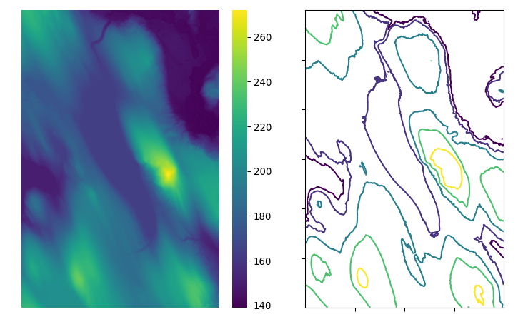
I sliced the data to an area that captured the lake and surrounding hills by visually determining the appropriate latitudes and longitudes. I then plotted a heatmap that illustrated the elevation range of the region (shown side-by-side with the contours below).

# x_start, x_end, y_start, and y_end determined visually
sub = df.loc[x_start:x_end, y_start:y_end]

f,ax = plt.subplots(figsize=(4,5), dpi=96)
# `.iloc[::5, ::5]` is optional and used to reduce the amount of data being plotted
sns.heatmap(sub.iloc[::5, ::5], square=True, xticklabels=False, yticklabels=False, ax=ax, cmap='viridis')

The last step was using matplotlib’s plt.contour() to slice the elevation into contours. I iterated on the number of slices and the elevation intervals, seeking to balance elevation fidelity with practical constraints like the number of total pieces and the absence of overly small pieces unable to be easily cut, stained, and glued. Once satisfied, I saved two copies of the contours as svg files for the next step, laser cutting.

# selected based on the heatmap to produce visually distinct contours
manual_contours = [152.4,164,187,210,233]

f,ax = plt.subplots(figsize=(10,10))
plt.contour(sub.columns, sub.index, sub, manual_contours, cmap='viridis')
ax.set_aspect(1)
ax.set_yticklabels('')
ax.set_xticklabels('')

# save as svg for laser cutting
f.savefig('output/contours.svg')

3. Laser cutting the wood pieces

For the following steps I originally used Illustrator, but today would use the free and open-source vector graphics editor Inkscape.

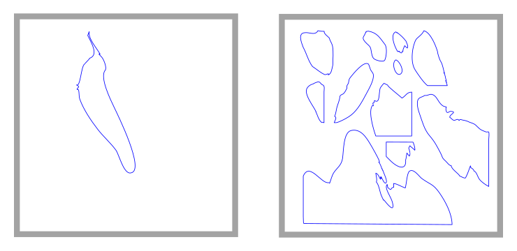
In the first svg file I deleted all contours except the central lake: this would be the template for the recessed epoxy fill and serve as the map’s base. To overcome some jagged points along the edge, I made liberal use of the Simplify path function (in Inkscape: Path -> Simplify; repeat as necessary). I then readied the file for upload to the laser cutting service Ponoko, which at the time (2017), had reasonably strict requirements of documents, such as requiring that all lines intended for cutting (as opposed to, for example, engraving) be blue and a specific stroke weight (screenshot below). As of this writing (2021), the document upload process is significantly smoother and has web-based interactivity.

In the second svg file, I removed the lake contour, deleted some small contours, and spatially separated the remaining elevation contours, again making liberal use of the path simplify function.

Lastly, I made sure that the svg scaling and dimensions were correct for the size I wanted. Having previously been a teaching assistant for an undergraduate design class at Stanford, I can still recall quite a few hilariously missized prints and cuts arising from insufficient attention to dimensions, most amusingly the inconsistent use of millimeters and inches.

4. Stain and glue the wood pieces

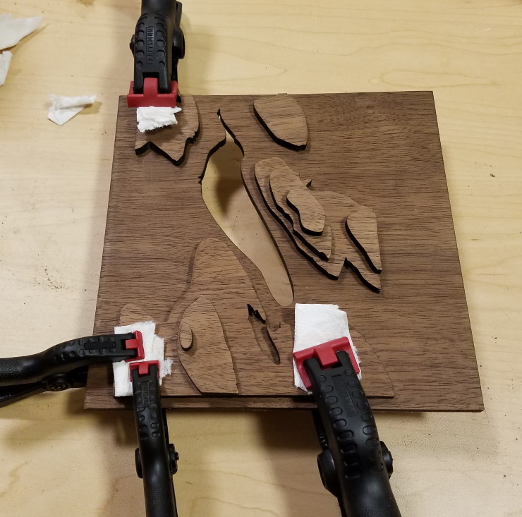
Careful not to overdue it because the wood was only a walnut veneer, I briefly sanded the pieces with increasingly fine grit sandpaper and applied a dark stain to accent the blues of the eventual lake water.

5. Pour the lake

My dad helped quite a bit here by providing ample advice as well as the epoxy, blue dye, and heat gun necessary to fill the lake into the recess. Thanks dad. My only recommendation looking back is to limit the generation of bubbles when stirring and pouring the epoxy in order to save on effort trying to remove them later with a heat gun or tooth pick.

Finished product

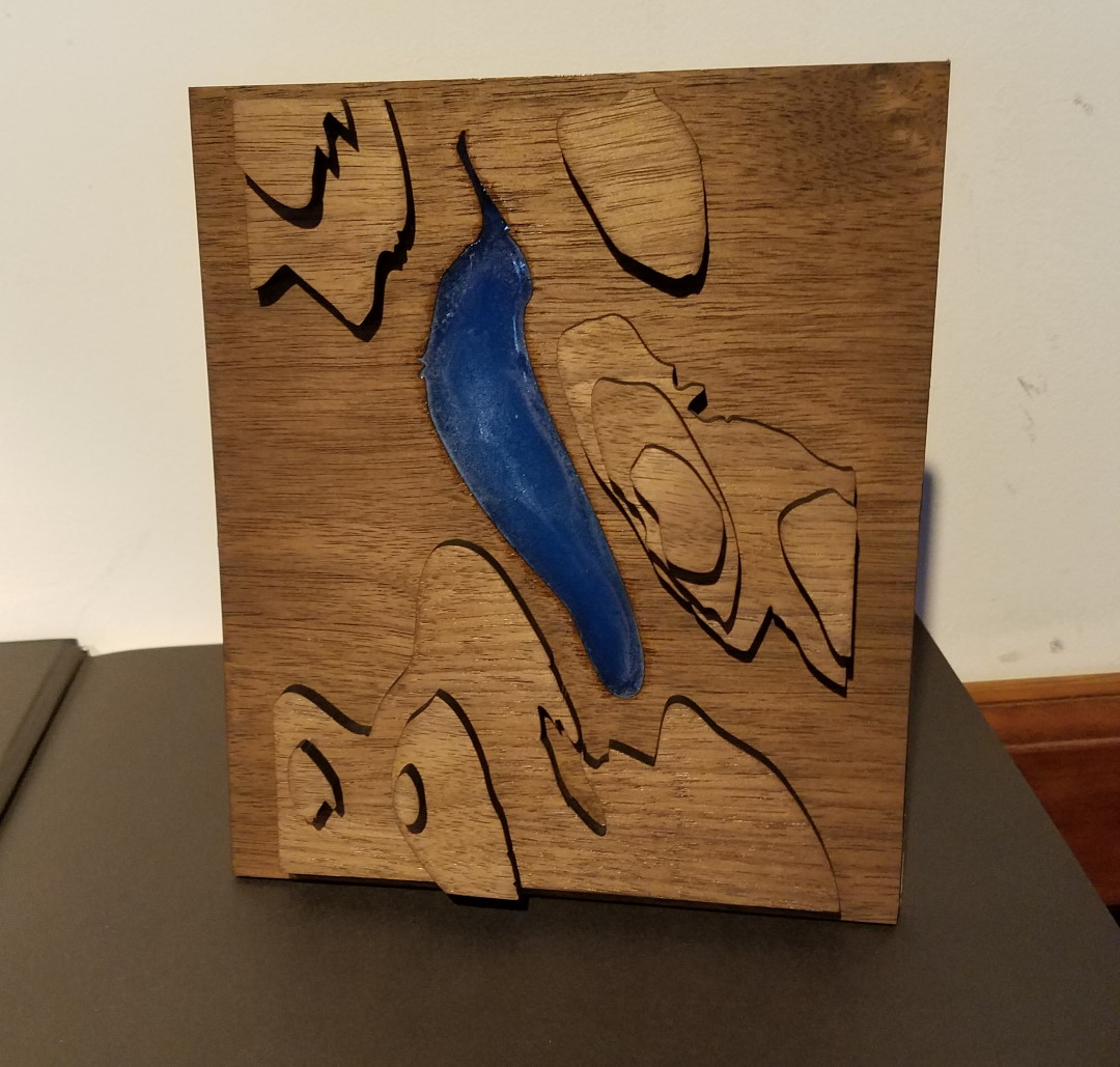
With an added stand, the final product:

Overall this was quite a fun project. It was not particularly expensive and was reasonably accessible using contract laser cutting, supplies available at a hardware store, and some basic graphics editing and python programming.

Footnotes

1. One year the flyer for this festival was itself a work of art, I wish I saved it.
2. This is a write-up of a project that I completed in 2017 while a graduate student.

Share on:

This work by Derek Croote is licensed under CC BY-NC 4.0